Sample Weighting with Conditional Random Fields
July 2022 update: The project described in this post resulted in three merged pull requests to AllenNLP:
- #5676 in allennlp: Implementation of Weighted CRF Tagger (handling unbalanced datasets)
- #341 in allennlp-models: Implementation of Weighted CRF Tagger (handling unbalanced datasets)
- #5638 in allennlp: FBetaMeasure metric with one value per key
These PRs were added to AllenNLP v2.10.0. Interestingly (or not :/), this was the last release before AllenNLP going on maintenance mode.
Conditional Random Fields (CRF) (original paper) is a popular probabilistic machine learning model that can deal with structured outputs. A CRF model is able, for instance, to predict variables over sequences or trees, such that the prediction algorithm takes into consideration dependencies among the elements of these structures (dependencies are given by the edges connecting the elements of a sequence or the nodes of a tree, for example). Consider, for instance, the NLP task of POS tagging, which consists of predicting the part of speech of each word in a given sentence (see figure below).
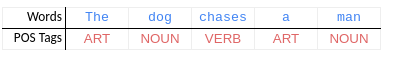
The ability to consider dependencies among elements of the output allows
a CRF model to learn (from data) that the tag VERB (the predicate of the sentence above)
is very likely to follow the tag NOUN (the subject),
or that the tag NOUN is very likely to follow the tag ART (article).
This is why we denote the outputs of such problems as structured outputs,
since the prediction of a variable may be dependent of the prediction of another variable.
This is not the case in the ordinary classification scenario
in which examples (and thus also the corresponding output variables) are assumed to be
independent and identically distributed (i.i.d.).
In this post, I discuss some approaches for sample weighting in CRF models. I present two naive approaches based on the scaling of emission and transition scores. I also implemented these two approaches, as well as the approach proposed by Lannoy et al. (2003), within the AllenNLP library. I then report on some simple experiments using the CoNLL NER datasets in order to compare the three approaches. The conclusion is that the simpler approaches result in a more meaningful result. I find the theoretical basis for Lannoy et al.’s approach tricky and hard to interpret. This seems to reflect on the achieved experimental results, although these experiments are quite limited.
Sample Weighting
One important technique employed in i.i.d. scenarios is sample weighting. In such technique, each example is weighted during training according to some criteria. One of the most common approaches consists of multiplying the loss function value for a training example by a weight. In a supervised i.i.d. scenario, we are given a set \(D=\{(x^{(1)},y^{(1)}), (x^{(2)},y^{(2)}), \ldots, (x^{(N)},y^{(N)})\}\) of \(N\) i.i.d. training examples, where \((x^{(i)},y^{(i)})\) is the \(i\)-th input-output training pair. Then, the weighted training loss function can be defined as:
\[\mathcal{L}_D(w) = \sum_{i=1,\ldots,N} c^{(i)} \cdot \mathcal L(y^{(i)}, f_w(x^{(i)}))\]where \(w\) is the set of parameters of the model \(f_w(x)\); \(\mathcal L(y^{(i)}, f_w(x^{(i)}))\) is the loss function applied on the model prediction for the \(i\)-th example; and \(c^{(i)}\) is an arbitrary weight for the \(i\)-th example. One common use case of sample weighting is to give higher weights for examples of underrepresented classes. In that way, one can lessen the undesired effects of unbalanced datasets. There are several other scenarios in which sample weighting have been successfully employed.
For CRF models, on the other hand, there is no standard approach to perform sample weighting based on the class of the examples. This is not straightforward because one example (a sentence, in the POS tagging example) comprises a set of output variables (a sequence of POS tags) and these variables are not i.i.d. This is the case due to the very nature of CRFs in which output variables are dependent on one another. As a consequence, the loss function used in CRFs cannot be independently factorized over the output variables and, thus, one cannot easily include a class-dependent weight in the loss function.
More than one year ago, a student in our research group in Brazil opened an issue in the AllenNLP github repository asking if their CRF implementation supported sample weighting. The short answer was no, but some of the library maintainers also said that they would be happy to include this functionality if someone would implement it. Dirk Groeneveld even pointed to a paper by Lannoy et al. (2012) in which a sample weighting for CRF was proposed. When I read the paper back then, I had the feeling that the theoretical motivation behind their approach was not correct. I thought it could work in practice but the motivation was just not right. But at that time we decided to change the course of the project and the new direction did not contemplate the weighted CRF. Now, after more than one year, I decided to give this task another try.
I implemented Lannoy et al.’s weighting approach and also two other simpler approaches based on the scaling of emission and transition scores. These later approaches are not novel. I have seen these ideas being mentioned at different places. I will denote these approaches emission and transition scaling. However, I do not know any report (or paper) on evaluating such approaches with a focus on the actual impact on performance for the weighted class. Thus, I performed some simple experiments using the CoNLL-2003 NER corpus in order to assess these three weighting approaches. In my experiments (again, quite simple), Lannoy et al.’s approach was not able to shift the performance of the model in a meaningful way. On the other hand, the emission and transition scaling approaches led to a clear shift on the performance of the weighted classes.
In this blog post, I present and discuss the results of these simple experiments. And before going into the experimental results, I briefly review CRF theory in the next section (you can skip it if you have a good knowledge about this model). Next, I describe the three weighting approaches. Then, I report on and discuss the experiments and, finally, I present some concluding remarks.
Linear-Chain CRF
CRF is a type of (undirected) graphical model, which means, very briefly, that it models the conditional dependencies among a set of random variables. The set of random variables includes the input and output variables for one specific example (for POS tagging, this would be the given sequence of words and the corresponding sequence of POS tags). As mentioned before, a CRF can model sequences but also other structures like trees, for instance. However, the linear-chain CRF (which models sequences) is the most common case, and this is the case I will be dealing with in this blog post.
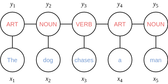
Given a sentence \(x=(x_1, x_2, \ldots, x_T)\) with \(T\) words, a CRF models the conditional probability \(p(y|x)\), where \(y=(y_1, y_2, \ldots, y_T)\) is the sequence of tags. In the figure below, you can see a representation of the graphical model for the exemplary sentence presented in the beginning of this post. In the top of the figure, there are the five outputs nodes \((y_1,y_2,\ldots,y_5)\), one for each tag. And in the bottom, there are the five input nodes \((x_1,x_2,\ldots,x_5)\), one for each word. An edge connecting a pair of nodes indicates a probabilistic dependency between them. For instance, there are edges connecting each consecutive tag node \((y_{t-1},y_t)\), for \(t=2,\ldots,5\), and edges connecting each tag node to its corresponding input node \((y_t,x_t)\), for \(t=1,2,\ldots,5\).
Trellis
The representation above is nice to visualize the linear structure of the model.
However, we are interested in modeling the discriminative model \(p(y|x)\),
so that we can, for instance, choose the most likely output sequence \(y^*\)
among the set of all possible sequences \(\mathcal{Y}\)
(more formally \(y^* = \arg\max_{y \in \mathcal{Y}} p(y|x)\)).
In order to define \(\mathcal{Y}\),
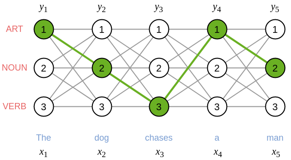
let us have a look at the figure below that represents the trellis of a CRF
for the given input sentence \(x\).
Now, remembering that \(y=(y_1, y_2, \ldots, y_T)\),
let us define that \(y_t \in \{1,2,\ldots,K\}\),
i.e. each tag \(y_t\) can take a value among \(K\) possible tags.
In our example, we consider only three tags: ART, NOUN and VERB
(we can represent each tag by an integer within \(\{1,2,\ldots,K\}\)).
In the figure, for each tag \(y_t\),
we have three possible nodes (since \(K=3\) in our example),
one for each tag.
The green nodes in the figure indicate the correct attribution of tags for the output sequence,
i.e., \(y_1=1\) (ART), \(y_2=2\) (NOUN), \(y_3=3\) (VERB), \(y_4=1\) (ART), and \(y_5=2\) (NOUN).
Finally, we can define \(\mathcal{Y} = \{1,2,\ldots,K\}^T\),
i.e., all possible sequences of \(T\) tags where each tag is taken from a set of \(K\) tags.
This means that each sequence of nodes in the trellis
(in each step \(t\), one node \(y_t\) is chosen from the \(K\) possibilities)
corresponds to a possible output sequence of tags \(y = (y_1,y_2,\ldots,y_T)\).
Transition and Emission Parameters
A CRF model is parametrized by two sets of parameters \(w=(\chi,\omega)\), where \(\chi=\{\chi_{kj}\} \in \mathbb{R}^{K \times K}\) are the transition parameters and \(\omega=\{\omega_{jp}\} \in \mathbb{R}^{K \times P}\) are the emission parameters. The transition parameters are employed in the transitions from a tag \(y_{t-1}\) to the next tag \(y_t\) (in the trellis above, each green edge is a transition for the considered sequence of tags \(y=(1,2,3,1,2)\)). There is a transition parameter \(\chi_{kj} \in \mathbb{R}\) for each possible transition from tag \(k\) to tag \(j\), for \(k,j \in \{1,2,\ldots,K\}\). Thus, to define the \(w\)-parameterized probability \(p(y|x;w)\) for the sequence of tags \(y=(1,2,3,1,2)\) represented in green in the trellis above, the parameters \(\chi_{12}, \chi_{23}, \chi_{31}, \chi_{12}\) will play a central role.
Let us not forget the input sequence \(x=(x_1, x_2, \ldots, x_T)\). We need to take it into account when defining \(p(y|x;w)\), so that this probability depends on the input words \(x_t\) (and their relations with the corresponding output tags \(y_t\)). In the trellis, we omit the edges between \(x_t\) and \(y_t\) to simplify visualization. But in the preceding figure, we represent these edges \((y_t,x_t)\). More specifically, each input word is represented by a vector of \(P\) features \(x_t = (x_{t1}, x_{t2}, \ldots, x_{tP}) \in \mathbb{R}^P\). Then, the emission parameters \(\omega=\{\omega_{jp}\} \in \mathbb{R}^{K \times P}\) of the CRF model are used to score the relationship between a tag \(y_t=j\) and a word \(x_t\) by means of the emission score function \(\omega(y_t,x_t)\) that is defined, for an arbitrary tag \(j\), as
\[\omega(j,x_t) = \langle \omega_j, x_t \rangle = \sum_{p=1,\ldots,P} \omega_{jp} \cdot x_{tp}\]where \(\omega_j\) is the \(j\)-th row vector of the emission parameters \(\omega \in \mathbb{R}^{K \times P}\) (i.e. the parameters used to weight the emission features for tokens tagged with the \(j\)-th tag: \(y_t = j\)), and \(\langle \omega_j, x_t \rangle\) is the inner product between \(\omega_j\) and \(x_t\).
Discriminative Conditional Probability
Equipped with these definitions, the discriminative conditional probability \(p(y|x;w)\) given by a CRF model parameterized by \(w=(\chi,\omega)\) will be proportional to the score \(s_w(x,y)\), that is \(p(y|x;w) \propto s_w(x,y)\). And this score function is defined as:
\[s_w(x,y) = \prod_{t=1}^T e^{\omega(y_t,x_t)} \cdot \prod_{t=2}^T e^{\chi(y_{t-1},y_t)}\]where \(\chi(k,j) = \chi_{kj}\) is simply the CRF parameter for a transition from tag \(k\) to tag \(j\). The score \(s_w(x,y)\) is the multiplication between two products: the product of the exponential of the emission scores for all tokens (\(e^{\omega(y_t,x_t)}\) for \(t=1,\ldots,T\)) and the product of the exponential of the transitions scores for all consecutive tokens (\(e^{\chi(y_{t-1},y_t)}\) for \(t=2,\ldots,T\)).
As mentioned above, we have that \(p(y|x;w) \propto s_w(x,y)\) (the probability of a tagging sequence is proportional to the score function). So, finally, we can define the probability \(p(y|x;w)\) as the normalized value of the score function:
\[p(y|x;w) = \frac{s_w(x,y)}{Z}\]where \(Z = \sum_{y' \in \mathcal{Y}} s_w(x,y')\). In other words, the conditional probability is equal to \(s_w(x,y)\) divided by the sum of the scores \(s_w(x,y')\) for all possible tagging sequences \(y' \in \mathcal Y\).
Learning a CRF and the Log-Loss Function
Given a training sample \((x,y)\), the learning problem can be defined as:
\[w^* = \arg\max_w p(y|x;w)\]that is, \(w^*=(\chi^*,\omega^*)\) are the parameters that, under the CRF model, result in the highest probability of the correct tagging sequence \(y\) given the input sequence \(x\).
One issue when implementing CRF is that the conditional probability is defined as a product of many small numbers. The product terms \(e^{\omega(y_t,x_t)}\) and \(e^{\chi(y_{t-1},y_t)}\) are probabilities (thus within \([0,1]\)) and, usually, are very small. If you keep multiplying small numbers, you will end up with underflow issues very quickly, unless you take appropriate measures. The most common measure to avoid such issues is to work on the log domain. Instead of computing \(w^*\) using the equation aforementioned, we can use the following equivalent equation:
\[w^* = \arg\max_w \log p(y|x;w)\]This function is denoted the log-likelihood and can be simplified as:
\[\begin{aligned} L(w) &= \log p(y|x;w) \\ &= \log \left( \frac{s_w(x,y)}{Z} \right) \\ &= \log s_w(x,y) - \log Z \end{aligned}\]And, due to the products of exponential functions, it can be further simplified as:
\[\begin{aligned} L(w) &= \log\left( \prod_{t=1}^T e^{\omega(y_t,x_t)} \cdot \prod_{t=2}^T e^{\chi(y_{t-1},y_t)} \right) - \log Z \\ &= \sum_{t=1}^T \omega(y_t,x_t) + \sum_{t=2}^T \chi(y_{t-1},y_t) - \log Z \end{aligned}\]The natural loss function of CRF is then the negative log-likelihood:
\[\mathcal L(w) = -L(w)\]So that to minimize the loss function corresponds to maximize the log-likelihood.
There are still issues to compute \(\log Z\),
but we can overcome them by applying another trick
(which involves the logsumexp function).
I will not go into more details about the learning algorithm for CRF here,
since it is not important to understand the weighting approaches.
Moreover, in case you are interested,
you can find many good resources online.
Nevertheless, I would like to give you a reference for a gem:
the lecture notes
by Prof. Jason Eisner.
Weighting Approaches
As mentioned in the beginning of this post, we care about sample weighting techniques which can give different weights for training samples according to the sample class. In the case of CRF models, this means attributing a weight \(c(y_t)\) to a token \(x_t\) according to its tag \(y_t\). Let us have a look at the log-likelihood equation again:
\[L(w) = \sum_{t=1}^T \omega(y_t,x_t) + \sum_{t=2}^T \chi(y_{t-1},y_t) - \log Z\]One problem is that you cannot factorize the log-likelihood of a CRF model (and, consequently, the loss function \(\mathcal L(w) = - L(w)\)) into terms that depend only on one individual \(y_t\). This is the case because of the structured characteristic of the linear-chain CRF, in which the conditional probability \(L(w)\) includes the transition terms \(\chi(y_{t-1},y_t)\).
Lannoy et al. Approach
Lannoy et al. (2012) argue that the main issue preventing the application of label weighting to CRF is the \(\log Z\) term, which is not given as a sum over \(t\), like the remaining terms of the log-likelihood. They then suggest that by using the scaling trick, instead of the log-domain trick, one is able to express \(\log Z\) as a sum over \(t\). The scaling trick consists of, in the forward algorithm, scaling the \(\alpha_t(k)\) terms at each time-step \(t\), such that they sum to 1.
\[\begin{aligned} z_t &= \sum_{k=1}^K \alpha_t(k) \\ \widehat \alpha_t(k) &= \frac{\alpha_t(k)}{z_t} \end{aligned}\]And then \(\log Z\) can be computed as the sum of the normalization factors over all time-steps:
\[\log Z = \sum_{t=1}^T \log z_t\]Finally, the log-likelihood equation can be rewritten as:
\[L(w) = \sum_{t=1}^T \omega(y_t,x_t) + \sum_{t=2}^T \chi(y_{t-1},y_t) - \sum_{t=1}^T \log z_t\]And, using this formulation, we can now include tag-dependent weights multiplying each term of the log-likelihood:
\[L(w) = \sum_{t=1}^T c(y_t) \cdot \omega(y_t,x_t) + \sum_{t=2}^T c(y_t) \cdot \chi(y_{t-1},y_t) - \sum_{t=1}^T c(y_t) \cdot \log z_t\]Criticism of Lannoy et al. Approach
Although I initially thought that this approach could work in practice, since the beginning, I did not agree with its theoretical justification. The most severe issue, in my opinion, is that there is no clear probabilistic interpretation for the terms \(\log z_t\). This means that it is quite hard to understand the impact of weighting these terms. In fact, one interpretation we can make about \(\log z_t\) is that it is related to all possible tags \(k \in \{1,\ldots,K\}\) at time-step \(t\) and not only to the correct tag \(y_t\). In order to understand this, we should consider that the role of the normalization term \(Z\) is to counter balance the score \(s(x,y)\). The latter is proportional to the probability that we want to maximize (the likelihood). But we need the normalization term to be sure that, by increasing the score \(s(x,y)\) of the correct tag sequence \(y\), we are increasing the probability of \(y\) and, at the same time, decreasing the probabilities of all incorrect tag sequences. Thus, \(\log Z\) and also \(\log z_t\) are related to all tags (the correct one and all the incorrect ones). To weight this term seems odd to me, and I cannot think of a meaningful interpretation for this weighting scheme.
Scaling of Emission Scores
As mentioned at the beginning of this post, one simple idea to implement sample weighting in CRF models consists in scaling the emission scores. This means simply multiplying the emission scores \(\omega(y_t,x_t)\) by the corresponding sample weight \(c(y_t)\). Then, instead of \(\omega(y_t,x_t)\), we use the following scaled version:
\[\overline \omega(y_t,x_t) = c(y_t) \cdot \omega(y_t,x_t)\]Observe that we scale only the emission score for the correct tag \(y_t\). It is also important to note that the scaled emission scores \(\overline \omega(y_t,x_t)\) are also used when computing \(\log Z\).
Scaling of Emission and Transition Scores
If you look at the loss function proposed by Lannoy et al. (2012), you can notice that the transition scores \(\chi(y_{t-1},y_t)\) are also scaled. I thus thought of trying a third sample weighting approach that scales the emission scores as well as the transition scores. To do that, one only needs to replace the original transition scores \(\chi(y_{t-1},y_t)\) by the following weighted version:
\[\overline \chi(y_{t-1},y_t) = c(y_t) \cdot \chi(y_{t-1},y_t)\]This seems a bit odd for me because you are scaling a term that depends on \(y_t\) but also on \(y_{t-1}\) with a \(y_t\)-dependent factor. But since Lannoy et al.’s approach does this, I decided to give it a try.
In the following section, I report on some simple experiments in order to understand the impact of these three approaches on the performance of the model, especially the performance regarding a weighted tag.
Experimental Evaluation
A robust evaluation of sample weighting approaches should
involve several tasks encompassing varying characteristics
(different domains, different levels of imbalance, etc.).
But here I present just a simple evaluation based on the popular
CoNLL-2003 NER task.
Additionally, I focus on weighting only two classes (one at a time):
person (PER) and location (LOC).
Although NER tasks are usually evaluated on an entity-level basis,
I will consider here a token-level evaluation.
The rationale is that the latter is more adherent to sample weighting
because the weights are attached to individual tokens and not to entities
(which can comprise more than one token).
Another modification I made was to remove the IOB prefix from the tags.
Thus, the tags B-PER and I-PER are converted to PER,
and B-LOC and I-LOC are converted to LOC,
as well as the tags related to the other entity types.
In the six figures below,
I present some performance metrics of the default CRF model in AllenNLP
while varying the weight of one tag (PER or LOC)
and using one of the three sample weighting approaches.
Observe that the weight axis (horizontal) is not scaled
(I find that equally spacing the labels is better in this case).
The figures in the first row correspond to the PER tag,
while the ones in the second row correspond to the LOC tag.
Regarding the three sample weighting approaches,
the first column corresponds to the emission score scaling,
the second column corresponds to the emission and transition score scaling,
and the third column corresponds to Lannoy et al.’s approach.
For each experiment, we report precision, recall and f-score of the weighted class,
and also the macro-averaged f-score.
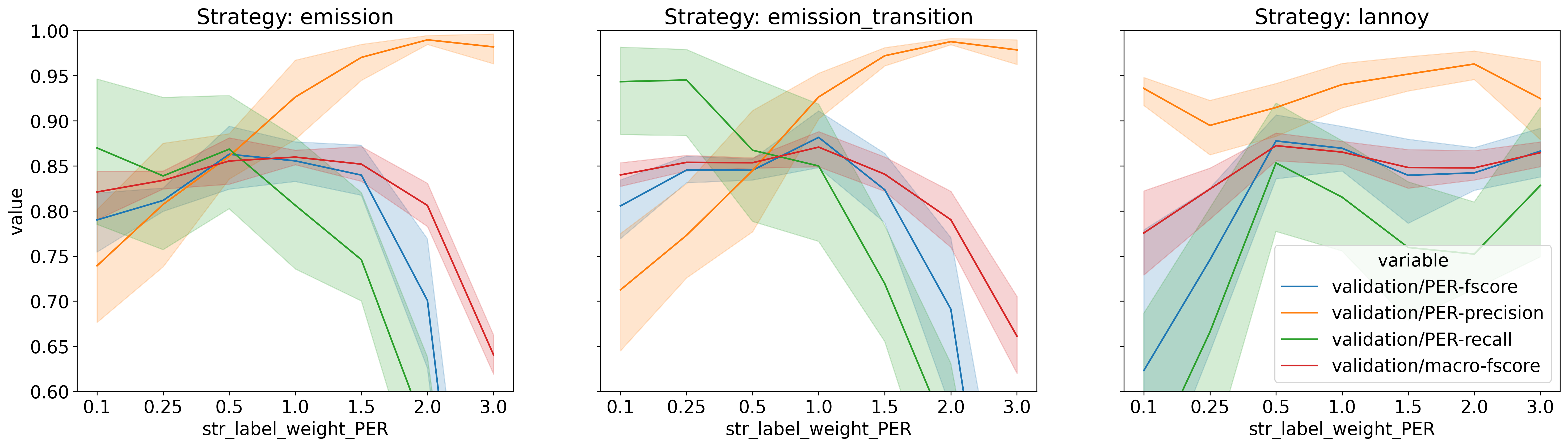
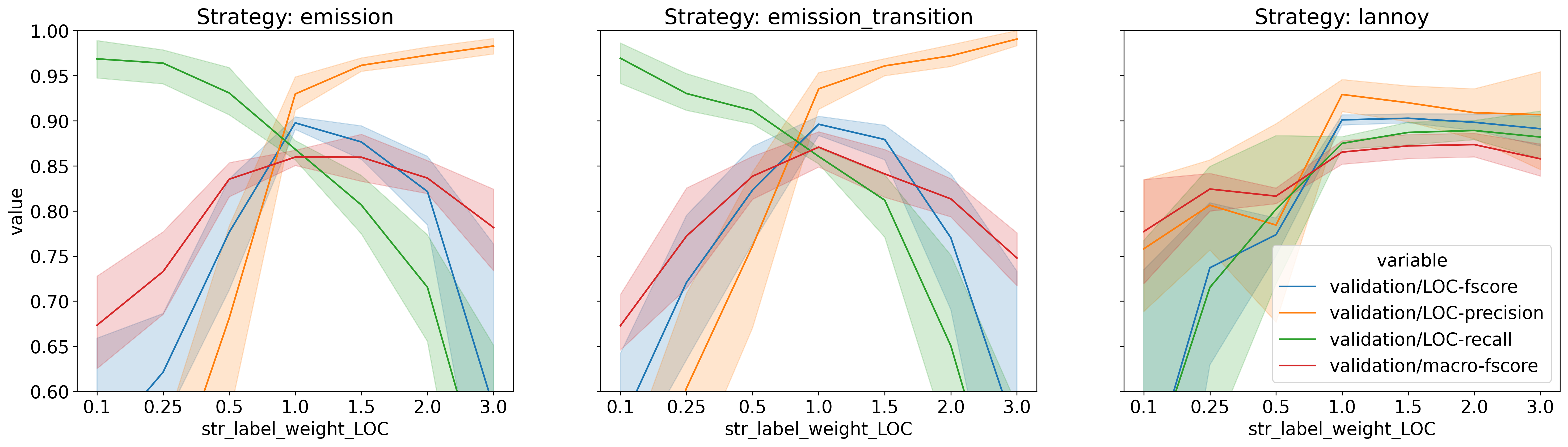
The first thing I would like to highlight is that the behavior of both the emission and the emission/transition weighting schemes are very similar. This is not surprising.
The most important thing to notice is the effect of the two simple weighting schemes (emission and emission/transition) on the precision and recall of the weighted classes. We can see that the precision increases with the weight of the tag, while the recall decreases with the weight of the tag. This is an interesting behavior because it allows us to control the tradeoff between precision and recall for one class. The f-score of the weighted class, as well as the macro-averaged f-score, goes down very quickly when the tag weight is increased or decreased very much. But this is usually unavoidable since the f-score is the harmonic mean of precision and recall (which means it is “attracted” more to the lower value between precision and recall).
Now, if we take a look at the results of Lannoy et al.’s approach (third column),
we see that precision and recall values for the weighted tag
do not follow an intuitive behavior.
The precision values for the tag PER, for instance,
goes down, then up, then down again,
while the tag weight is monotonically increased.
On the other hand, the recall values follow an inverse pattern.
In the case of the tag LOC,
the precision and recall values present a different pattern
than the one for tag PER.
This unintuitive behavior makes the use of this method difficult,
since it is hard to understand or predict the expected behavior.
Concluding Remarks
In this post, I discussed some approaches for sample weighting in CRF models. I presented two naive approaches based on the scaling of emission and transition scores. I also implemented these two approaches, as well as the approach proposed by Lannoy et al. (2003), within the AllenNLP library. I then performed some simple experiments using the CoNLL NER datasets in order to compare the three approaches. The conclusion is that the simpler approaches result in a more meaningful result. I find the theoretical basis for Lannoy et al.’s approach tricky and hard to interpret. This seems to reflect on the achieved experimental results, although these experiments were quite limited.
I plan to submit a pull request to the AllenNLP library with the implemented approaches. If I was to choose one of the three approaches, I would choose the emission-based one. It is the simplest among the three and achieves good results. I will update this post with further information and links to the PR. (See update in the beginning of the post.)